

To help customers with filter selection, we generally provide a lot of information on what our filters can do. But in this new Filter Basics Series, we are taking a step back to cover some background information on how filters do what they do. Regardless of the technology behind the filter, there are several key concepts that all filters share that we will dive into throughout this series. By providing this detailed fundamental filter information, we hope to help you simplify your future filtering decisions.
In part 11, the last post in our Filter Basics series, we review the information S-parameters can tell you about a filter’s performance and show an example of how to plot a filter’s S-parameters using a free open-source tool.
In general, we like to think of scattering parameters, commonly known as S-parameters, as the Swiss Army knife of RF data since this data can tell you quite a bit about the performance of a filter. This is because an S-parameter file refers to the scattering matrix of a microwave network, which is a mathematical construct that quantifies how RF energy propagates through a linear multi-port network.
For a two-port network, the S-parameter matrix consists of four S-parameters – S11, S12, S21, and S22 –that define the relationships between the two ports in the RF system. More specifically, these four S-parameters define the following elements in the bidirectional network:
- S11 – The reflection coefficient (𝛤) at the input, related to return loss
- S12 – A transmission coefficient that defines reverse gain
- S21 – Also a transmission coefficient that measures forward gain – in the case that the measurement ports have the same impedance, this is a measure of insertion loss
- S22 – Also a reflection coefficient, defines output port reflection
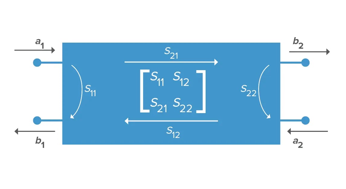
Figure 1. A representation of an S-parameter matrix of a two-port RF device where a represents an input and b represents an output.
Using the S-parameters for a filter, you can calculate values for insertion loss, return loss, and voltage standing wave ratio (VSWR), which is a measure of the filter’s match to a given impedance, with the following equations:
| Insertion Loss | Return Loss | VSWR |
| RL = -20Log 𝛤 |
A Real-World Example of Plotting a Filter’s S-Parameters
Let’s now look at an example of how to measure a filter’s performance using the S-parameter file for one of our catalog filters, the B095MB1S, which is a 9.5 GHz surface mount bandpass filter. For the analysis in this example, we will use a free open-source tool, scikit-rf, which is based on the Python programming language, to plot the S-parameters.
To access the S-parameter file for this filter (or any of our filters), just search for the filter on our website. Once you have the file, store it on your computer in a location where it is easy to access from within your Jupyter setup (which is a tool that makes it easier to write Python code interactively in a local web browser). We recommend renaming the file with a name that is easy to recognize. For our example, we put the file in a folder called ‘xband2’ and named the file ‘B095MB1S.s2p.’ Since Jupyter can see this folder, we can make a Network and review the Network properties. Below is the Python code we input in Jupyter to call this S-parameter file and create this example Network as well as the results.
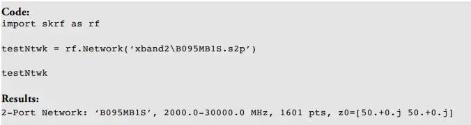
Note that in this example, the testNtwk is a Network object representing a two-port Network. The summary information in the results tells us the frequency range of this data set, the number of data points, and the impedance of the Network. The Network class also comes with convenient built-in methods for plotting and manipulating data. In this example, we can quickly plot the log-magnitude in decibels for the filter’s frequency range for four standard S-parameters by calling the plot_s_db method, or we can plot each s-parameter individually (Figures 2 and 3).
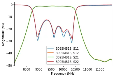 Figure 2. All Four S-parameters in one plot.
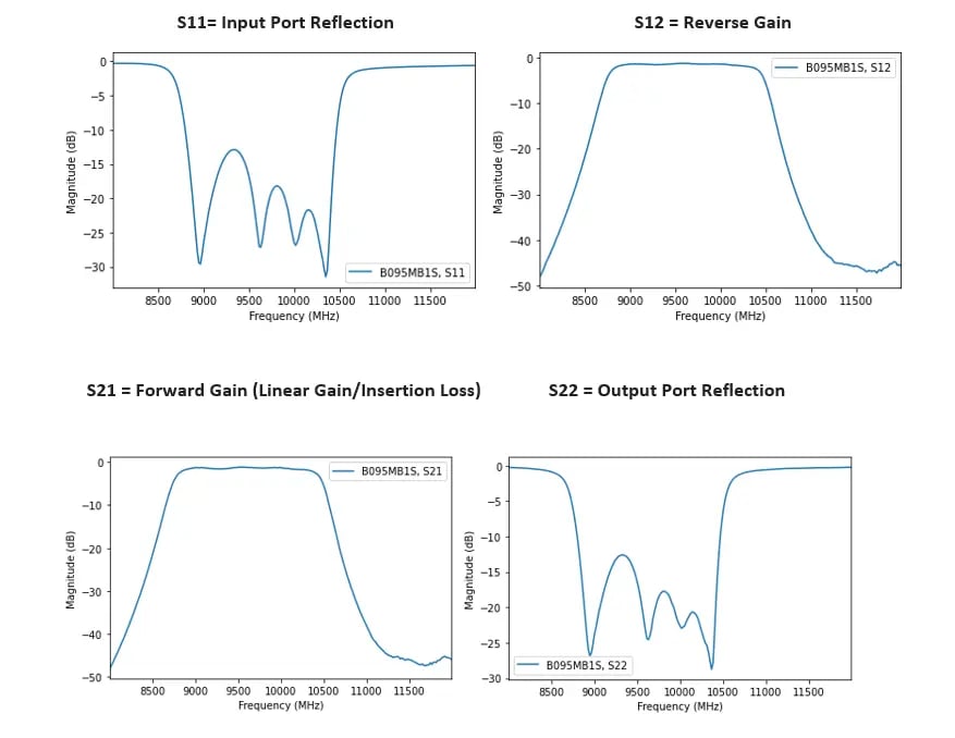
Figure 3. Each S Parameter plotted individually.
This post concludes our 11-part Filter Basics series. Now that you have a better understanding of how filters work, we would love to hear from you to learn more about your application needs and how we can help you with filter selection for your next application.
Ready to take a deeper dive in the fundamentals of RF Filters? Download the comprehensive Filter Basics guide today.