

To help customers with filter selection, we generally provide a lot of information on what our filters can do. But in this new Filter Basics Series, we are taking a step back to cover some background information on how filters do what they do. Regardless of the technology behind the filter, there are several key concepts that all filters share that we will dive into throughout this series. By providing this detailed fundamental filter information, we hope to help you simplify your future filtering decisions.
In part 7 of this series, we perform a deep dive on the different ways you can think about Q factor for the components going into your filter or your filter as a whole.
As an RF engineer, you likely frequently hear the term “quality factor”, or Q factor, used as shorthand figure of merit (FOM) for RF filters. In short, Q factor is expressed as the ratio of stored versus lost energy per oscillation cycle.
More specifically, Q factor generally describes specifications such as the steepness of skirts, or the selectivity, and how low the insertion loss is. Overall losses through a resonator increase as Q factor drops and will increase more rapidly with frequency for lower values of resonator Q. However, truly understanding how Q factor is determined is a bit more intricate. Let’s start by looking back to the example bandpass filter specification we showed in Part 3.
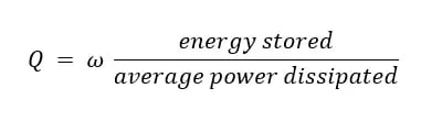
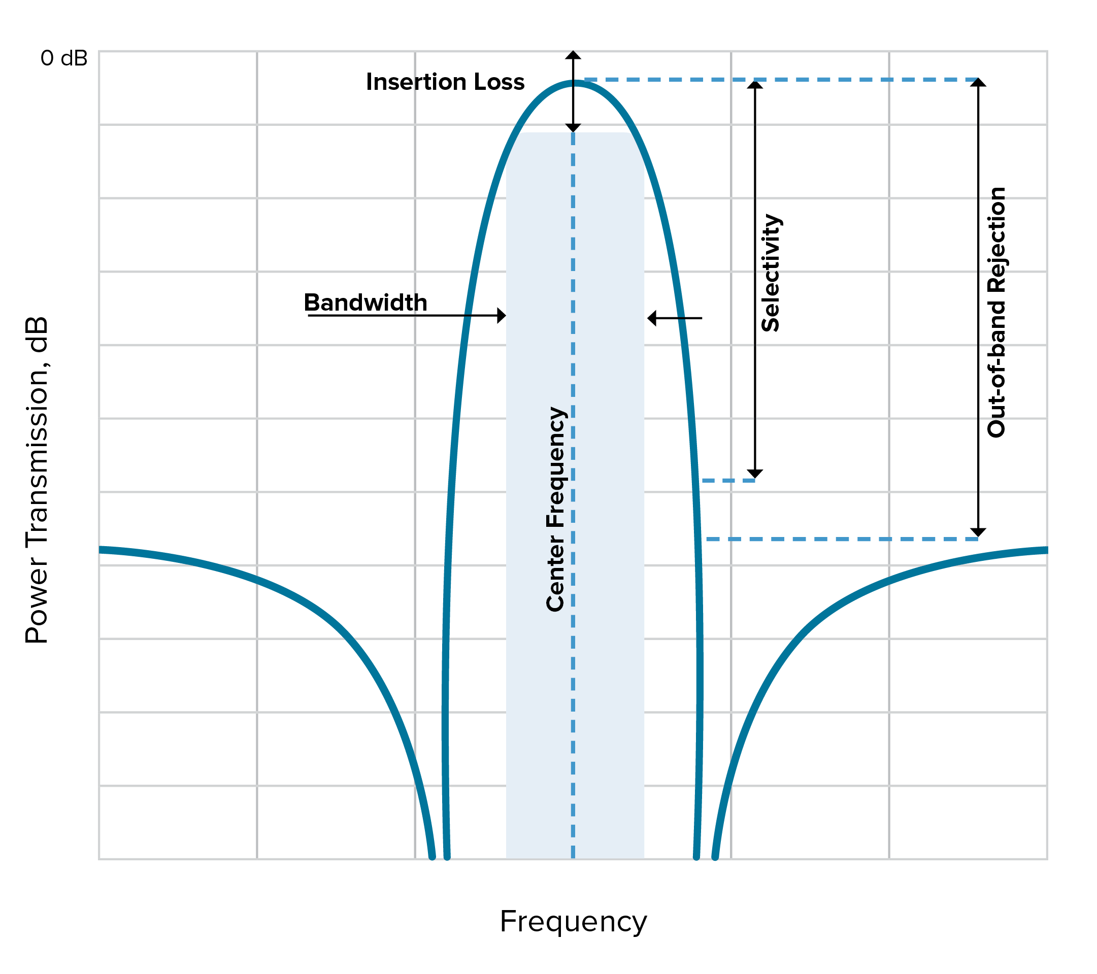
Figure 1. An example of a typical bandpass filter response.
In this example, the X axis shows the operating frequency of the bandpass filter while the Y axis shows the power allowed through the filter in decibels. We can mark the following characteristics of this filter on this graph:
- Center frequency – The geometric or arithmetic mean of the upper and lower cutoff frequencies or 3dB points of the bandpass filter.
- Bandwidth – Usually taken from the 3dB points on either side of the center frequency.
- Insertion loss – Drawn here as the loss at the center frequency. In general, when someone says high Q in reference to insertion loss, this usually means low insertion loss.
- Selectivity – This is a measurement of a filter’s ability to pass or reject specific frequencies closer to the band of interest. This is what people usually mean when they talk about ‘steep skirts’ or a ‘sharp response.’ Generally, high Q means high selectivity.
Understanding the Different Components of Q Factor
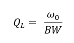
There are three types of Q – loaded (QL), unloaded Q (Qu), and external Q (Qe) that make up Q factor. QL is measured by looking at a plot of a filter’s performance. The standard definition of QL is as a FOM for bandwidth calculated with the following equation: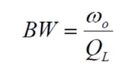
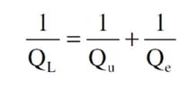
QL is driven by what goes on inside the filter, which is the Qu, and the way that the device is coupled to the external world, which is the Qe:
In general, QL is a convenient way to talk about a filter’s performance as plotted. But when it comes to what makes a filter work the way it does, it’s best to look at the QU of the resonators the filter is built up from. Now let’s look more specifically at three different ways to define Q factor using the different types of Q.
Three Ways to Define Q Factor
As mentioned, there are actually a few different ways to define Q factor, depending on the context of the discussion. This includes the following:
- Bandpass Q Factor – This talks about the width of a filter. Sometimes this is QL ,as discussed above, but with wide filters it is tricky to use Bandpass Q Factor
- Component Q Factor – Addresses individual inductor or capacitor Q
- Pole Q Factor – Tells us about the performance of different parts of a filter response, and is more abstract and based on Pole Zero Plots
While component and bandpass Q are the two most common types of Q factor referenced, let’s further explore the context of all three to better understand what someone may mean when they say a filter or component has “high Q.”
Bandpass Q Factor
When connecting components to create a resonant circuit, we need to look at QL, which for bandpass filters is referring to selectivity as shown in Figure 2.
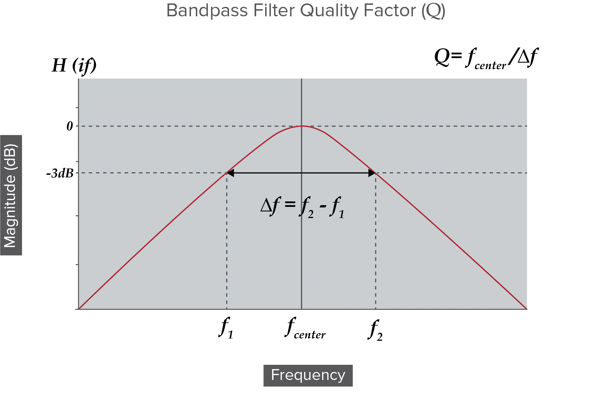
Figure 2. A graph showing bandpass filter Q Factor.
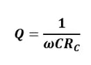
If the resonant circuit has Bandpass properties, we can define QL with the following formula:
 It is important to note that this approach works for narrowband filters. However, when f1 and f2 are widely separated, which usually means two octaves or more between f1 and f2, this results in a wideband with the filter often constructed by combining a high pass filter for f1 and a low pass filter for f2. In this situation it might make sense to think about the pole quality factor instead, which we will discuss later in this post, or to look at the performance of the high pass and low pass sections and look at their QL.
Component Q Factor
As mentioned, component Q factor looks at just the component, such as the inductor or capacitor, in isolation from the rest of the circuit. Components have Qu related to the component values and loss. Since inductance and capacitance provide an opposition to AC that is measured in terms of reactance, let’s look at Q in terms of how the component behaves under reactance.
For a reactance with no loss: 
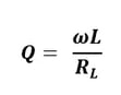
For an Inductive reactance, Q increases with frequency and decreases with loss as shown in the formula below.
 For capacitive reactance, Q decreases with frequency and with loss as shown in the formula below.
More specifically, the Q of an individual reactive component depends on the frequency at which it is evaluated, which is typically the resonant frequency of the circuit that it is used in. The formula for Q depends on whether we imagine the R to be in series with or in parallel with the reactance. The following formulas can be used to calculate Qu:
Inductive Reactance: 
Capacitive Reactance: 
R in series with X: 
R in parallel with X: 
Pole Q Factor
For more complex systems such as wider filters, we can look at the Pole Q factor, which tells us about the performance of different parts of the filter response. A filter has a transfer function 𝐻(𝑠) which tells us what an output signal will look like for a given input signal.
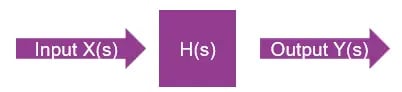
Filter Transfer Functions are expressed in terms of the complex variable ‘s’ because some problems are much easier to solve in the Laplace domain than they are in the time domain. The output signal Y(s) can be converted back into real numbers, and we can see how a filter’s performance is determined by the structure of the transfer function H(s). We can find the values for s for when the transfer function either gets large because the denominator heads to zero, or gets small because the numerator heads to zero.
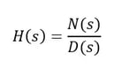
When N(s) heads to zero we call these values of s ‘zeros’ because the transfer function tends to get smaller. When D(s) heads to zero we call these values of s “poles” because the transfer function tends to get larger. In the Pole Zero Plot in Figure 3, you can see that the poles are marked with an X.
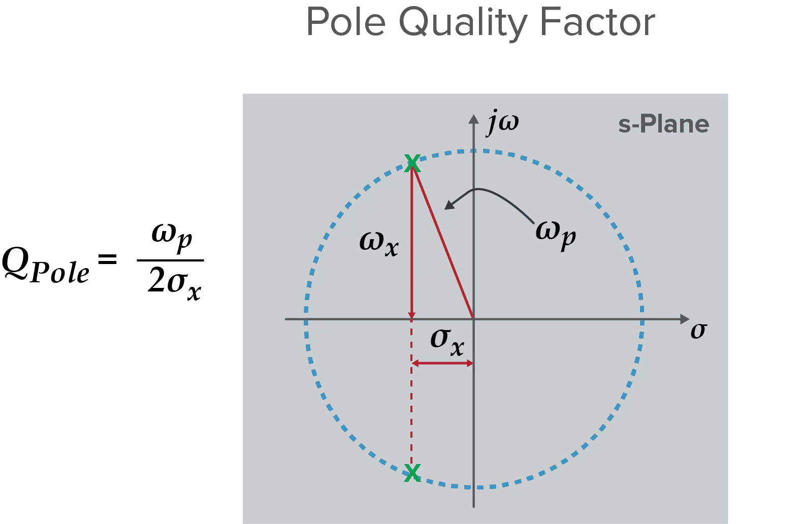
Figure 3. A Pole Zero Plot that shows Pole Q factor.
In this plot there are two poles that are complex conjugate pairs. The length of the arrow from the origin to the X is the frequency ωp. The distance along the real axis can be written in terms of the Q factor:
 Poles and zeros come from analyzing the system as a whole. Poles close to the y axis enhance amplitude response, making that part of the filter “sharp,” which is one of the ways Q factor drives selectivity. Additionally, based on this plot, high Q for a pole means low sigma. Since earlier we said this real component has to do with damping, which in turn is related to energy loss of a resonator, this makes sense.
In the next post in this series, we will get more into the specifics of bandwidth.
Ready to take a deeper dive in the fundamentals of RF Filters? Download the comprehensive Filter Basics guide today.